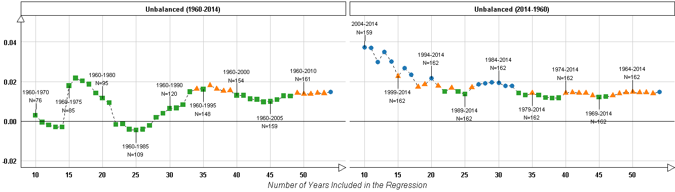
This article analyzes a unique panel data set to assess the effect of militarism on per capita carbon dioxide emissions. We extend previous research examining the effects of military expenditures on carbon emissions by including in our analyses over 30 years of additional data. In addition, we compare our preliminary results to those obtained from other estimation procedures. Specifically, we report and visually illustrate the results of 54 cross-sectional models (one for each year) and 36 unique panel regression models on both balanced and unbalanced panels. We assess how this relationship has changed over time by testing for interactions between military spending and time and by systematically re-analyzing our data across 180 panel regressions with varying time frames. A strong and enduring association between military spending and per capita carbon emissions is indicated in cross-sectional comparisons. Our panel analyses reveal a much weaker and varying relationship that has become stronger in recent decades. Moreover, we find that the effect of military spending on per capita carbon emissions is moderated by countries’ level of economic development, with military spending of more wealthy countries having relatively larger net effects on carbon emissions. We partially confirm previous findings on the temporal stability of the environmental impacts of militarism. Our analyses show, however, that this temporal stability has emerged relatively recently, and that the relationship between military expenditures and carbon emissions is weaker prior to the 1990s.