A new article has just been published in the Journal of Criminal Justice, “The prevalence of fatal police shootings by U.S. police, 2015–2016: Patterns and answers from a new data set” by Shane, Lawton, and Swenson (2017) .
The authors make some good points that I mostly agree with, but I cannot make sense of their finding that the mean rate of black civilians killed by police (per 100,000) is lower than that of whites. The finding is reported in Table 3 and in the discussion of their descriptive statistics:
“The mean rate for Blacks was lower than for Whites, Hispanics (p < 0.000) and Native Americans (p < 0.002), but was not different for Asians and others” (3)
“The mean rate of fatalities for Whites (M =0.741) is significantly lower than for Hispanics (M = 0.897; p < 0.000) and Native Americans (M = 1.106; p < 0.005), but is higher than for Blacks (M=0.633; p < 0.000).” (5)
Their data come from the Washington Post and covers 2015-2016. They aggregate deaths by state and calculate the “mean fatality rate per 100,000 population (based on 2016 U.S. Census Bureau state populations).”
From everything I’ve read and the data I’ve examined, when normalized by race-specific population, the black rate of police shooting deaths is higher than that for whites, at the aggregate national level. You can look at this data yourself with an online R Shiny App I created here:
https://johnbradford.shinyapps.io/policeshooting/
So I decided to examine the Washington Post data again, calculating the fatality rate for each racial group for each state. The code and results are posted below.
I. Load Washington Post Data.
First, we have to load the necessary R packages and Washington Post data. I include at the beginning a function for returning state abbreviations from state names regardless of capitalization or punctuation. I also filter to exclude cases after 2016.
getState.abb <- function(x) {
    ## remove punctuation and twim white space, convert to lower case
    x <- tolower(trimws(gsub("[[:punct:]]", "", x)))
    x[which(x == "washington dc")] <- "district of columbia"

    states.abb <- c(state.abb, "DC", "DC", "PR")
    states.name <- c(state.name, "District of Columbia", "District of Columbia",
        "Puerto Rico")

    m.abb <- tolower(states.abb)
    m.name <- tolower(gsub("[[:punct:]]", "", states.name))

    x[which(x %in% m.abb)] <- states.abb[match(x[which(x %in% m.abb)], m.abb)]
    x[which(x %in% m.name)] <- states.abb[match(x[which(x %in% m.name)], m.name)]

    return(x)
}


library(dplyr)
library(readr)

wapo <- read_csv("https://cdn.rawgit.com/washingtonpost/data-police-shootings/master/fatal-police-shootings-data.csv") %>%
    dplyr::transmute(Race = race, Race = replace(Race, which(Race == "W"), "White"),
        Race = replace(Race, which(Race == "B"), "Black"), Race = replace(Race,
            which(Race == "H"), "Hispanic"), Race = replace(Race, which(Race ==
            "A"), "Asian"), Race = replace(Race, which(Race == "N"), "Native American"),
        Race = replace(Race, which(Race == "O"), "Other"), year = as.numeric(format(date,
            "%Y")), State = getState.abb(state)) %>% ## Sum across years for state for each race
dplyr::filter(year < 2017) %>% dplyr::group_by(State) %>% dplyr::summarise(killed.White = length(which(Race ==
    "White")), killed.Black = length(which(Race == "Black")), killed.Hispanic = length(which(Race ==
    "Hispanic")), killed.Asian = length(which(Race == "Asian")), killed.NativeAmerican = length(which(Race ==
    "Native American")), killed.Total = n())

knitr::kable(wapo)| State | killed.White | killed.Black | killed.Hispanic | killed.Asian | killed.NativeAmerican | killed.Total |
|---|---|---|---|---|---|---|
| AK | 5 | 0 | 0 | 0 | 5 | 11 |
| AL | 28 | 12 | 0 | 0 | 0 | 42 |
| AR | 13 | 3 | 0 | 0 | 0 | 20 |
| AZ | 47 | 3 | 29 | 0 | 8 | 92 |
| CA | 98 | 55 | 134 | 13 | 0 | 327 |
| CO | 28 | 7 | 17 | 2 | 1 | 60 |
| CT | 5 | 0 | 1 | 0 | 0 | 6 |
| DC | 0 | 9 | 0 | 0 | 0 | 9 |
| DE | 3 | 1 | 0 | 0 | 0 | 4 |
| FL | 54 | 42 | 16 | 1 | 0 | 120 |
| GA | 26 | 19 | 5 | 1 | 0 | 55 |
| HI | 0 | 1 | 0 | 1 | 0 | 8 |
| IA | 7 | 3 | 0 | 0 | 0 | 10 |
| ID | 10 | 0 | 3 | 0 | 0 | 13 |
| IL | 14 | 28 | 5 | 0 | 0 | 47 |
| IN | 19 | 10 | 2 | 0 | 0 | 33 |
| KS | 16 | 1 | 2 | 0 | 0 | 19 |
| KY | 25 | 6 | 2 | 0 | 0 | 34 |
| LA | 18 | 25 | 0 | 1 | 0 | 46 |
| MA | 9 | 7 | 5 | 0 | 0 | 21 |
| MD | 8 | 21 | 0 | 0 | 0 | 30 |
| ME | 3 | 0 | 0 | 0 | 0 | 4 |
| MI | 17 | 11 | 1 | 0 | 0 | 29 |
| MN | 17 | 5 | 1 | 1 | 0 | 26 |
| MO | 24 | 15 | 1 | 0 | 0 | 42 |
| MS | 11 | 5 | 0 | 0 | 0 | 16 |
| MT | 9 | 0 | 0 | 0 | 0 | 9 |
| NC | 32 | 21 | 1 | 1 | 0 | 56 |
| ND | 1 | 0 | 0 | 0 | 1 | 2 |
| NE | 12 | 3 | 0 | 0 | 0 | 15 |
| NH | 5 | 0 | 0 | 0 | 0 | 5 |
| NJ | 10 | 11 | 3 | 1 | 0 | 27 |
| NM | 15 | 0 | 24 | 0 | 1 | 41 |
| NV | 15 | 5 | 10 | 0 | 0 | 33 |
| NY | 16 | 17 | 1 | 1 | 0 | 36 |
| OH | 25 | 24 | 0 | 2 | 0 | 55 |
| OK | 35 | 13 | 4 | 0 | 0 | 58 |
| OR | 26 | 2 | 0 | 0 | 0 | 30 |
| PA | 17 | 18 | 1 | 0 | 0 | 40 |
| RI | 0 | 1 | 1 | 0 | 0 | 2 |
| SC | 23 | 13 | 0 | 0 | 0 | 36 |
| SD | 5 | 0 | 0 | 0 | 2 | 7 |
| TN | 28 | 7 | 2 | 1 | 0 | 42 |
| TX | 82 | 35 | 52 | 1 | 1 | 180 |
| UT | 17 | 0 | 0 | 0 | 0 | 18 |
| VA | 15 | 18 | 2 | 0 | 0 | 35 |
| VT | 2 | 0 | 0 | 0 | 1 | 3 |
| WA | 25 | 4 | 4 | 2 | 4 | 42 |
| WI | 19 | 7 | 2 | 0 | 0 | 28 |
| WV | 16 | 3 | 0 | 0 | 0 | 22 |
| WY | 5 | 0 | 1 | 0 | 1 | 8 |
II. Load Census Data
Next, we have to load the state-level population data by race. They use 2016 Census data, but we should get similar results from the 2015 Census Data, which would just as legitimate anyway since the Wasghinton Post data covers 2015 and 2016. The census data can be retrieved online:
Using this data, you can also normalize by gender, age, and race and their cross-tabulations. Below I only examine race. The state names also have to be abbreviated to match the Washington Post data.
library(dplyr)
library(tidyr)
library(readr)

census_state <- read_csv("https://www2.census.gov/programs-surveys/popest/datasets/2010-2015/state/asrh/sc-est2015-alldata5.csv") %>%
    ## filtering to include both males and females
dplyr::filter(SEX == 0) %>% ## selecting only 2015 data, renaming the columns
dplyr::transmute(State = NAME, Hisp = ORIGIN, Race = RACE, AGE = AGE, population = POPESTIMATE2015) %>%
    ## Creating Race categories - 'Hispanics' are Hispanic Whites.  But the
## results are roughly the same if you include hispanic blacks, asians, etc.
## since there are so few of them.  I'm also combining Asians and PAcific
## Islanders since they are not distinguished in the WaPo data.
dplyr::mutate(State = getState.abb(State), Race = replace(Race, which(Race ==
    1 & Hisp == 1), "White"), Race = replace(Race, which(Race == 1 & Hisp ==
    2), "Hispanic"), Race = replace(Race, which(Race == 2 & Hisp == 0), "Black"),
    Race = replace(Race, which(Race == 3 & Hisp == 0), "Native American"), Race = replace(Race,
        which(Race == 4 & Hisp == 0), "Asian"), Race = replace(Race, which(Race ==
        5 & Hisp == 0), "Asian")) %>% dplyr::select(-c(Hisp)) %>% dplyr::filter(Race %in%
    c("White", "Hispanic", "Black", "Asian", "Native American")) %>% dplyr::group_by(State,
    Race) %>% ## Summing across all ages each race within each state
dplyr::summarise(population = sum(population, na.rm = T)) %>% tidyr::spread(Race,
    population) %>% ## Creating a 'Total' population category
dplyr::mutate(Total = White + Hispanic + Black + Asian + `Native American`)

knitr::kable(census_state)| State | Asian | Black | Hispanic | Native American | White | Total |
|---|---|---|---|---|---|---|
| AK | 74220 | 40105 | 41640 | 143826 | 496799 | 796590 |
| AL | 92339 | 1338287 | 175866 | 66733 | 3268304 | 4941529 |
| AR | 69177 | 490231 | 197047 | 58338 | 2226051 | 3040844 |
| AZ | 331963 | 403715 | 1935766 | 429351 | 3930262 | 7031057 |
| CA | 6869486 | 2989322 | 14040493 | 1078986 | 15788764 | 40767051 |
| CO | 255130 | 304298 | 1068750 | 148150 | 3855642 | 5631970 |
| CT | 197283 | 466878 | 473242 | 40962 | 2500213 | 3678578 |
| DC | 37653 | 335822 | 55945 | 9141 | 254510 | 693071 |
| DE | 44550 | 228005 | 70669 | 12698 | 615841 | 971763 |
| FL | 766873 | 3642783 | 4622640 | 203379 | 11482439 | 20718114 |
| GA | 491234 | 3364359 | 820463 | 112516 | 5650933 | 10439505 |
| HI | 1173481 | 56565 | 101049 | 37862 | 524496 | 1893453 |
| IA | 92785 | 140006 | 164384 | 31348 | 2754083 | 3182606 |
| ID | 44902 | 22007 | 187076 | 46816 | 1395356 | 1696157 |
| IL | 810389 | 2009937 | 2025465 | 139840 | 8132912 | 13118543 |
| IN | 179317 | 712550 | 402399 | 62546 | 5400383 | 6757195 |
| KS | 109477 | 222885 | 309984 | 68432 | 2290079 | 3000857 |
| KY | 86311 | 413580 | 135678 | 36636 | 3837964 | 4510169 |
| LA | 110022 | 1559188 | 200763 | 63567 | 2817869 | 4751409 |
| MA | 512363 | 659668 | 618260 | 70214 | 5101413 | 6961918 |
| MD | 463421 | 1926573 | 478070 | 76800 | 3241665 | 6186529 |
| ME | 23323 | 26532 | 18654 | 19660 | 1264763 | 1352932 |
| MI | 366630 | 1530388 | 432381 | 153104 | 7688454 | 10170957 |
| MN | 313841 | 393395 | 252291 | 117564 | 4554134 | 5631225 |
| MO | 166654 | 783917 | 222123 | 82875 | 4969582 | 6225151 |
| MS | 43864 | 1146449 | 76423 | 30132 | 1734474 | 3031342 |
| MT | 16435 | 11400 | 30771 | 86007 | 917350 | 1061963 |
| NC | 358676 | 2348191 | 778108 | 229119 | 6560680 | 10274774 |
| ND | 15364 | 23131 | 22546 | 49847 | 662513 | 773401 |
| NE | 58998 | 113682 | 178335 | 39891 | 1547639 | 1938545 |
| NH | 43327 | 27973 | 40507 | 11838 | 1230066 | 1353711 |
| NJ | 956570 | 1439670 | 1521368 | 100180 | 5146692 | 9164480 |
| NM | 56475 | 69601 | 939053 | 246717 | 829130 | 2140976 |
| NV | 346130 | 311617 | 744673 | 77354 | 1544500 | 3024274 |
| NY | 1948015 | 3786724 | 2910344 | 318526 | 11356124 | 20319733 |
| OH | 310274 | 1634412 | 358475 | 101965 | 9476886 | 11882012 |
| OK | 121260 | 364882 | 342672 | 532016 | 2797325 | 4158155 |
| OR | 265197 | 120634 | 465792 | 136727 | 3203032 | 4191382 |
| PA | 513870 | 1653996 | 702016 | 107484 | 10088820 | 13066186 |
| RI | 48117 | 100579 | 120418 | 18738 | 799027 | 1086879 |
| SC | 107421 | 1404522 | 230290 | 53394 | 3193778 | 4989405 |
| SD | 16539 | 21594 | 24718 | 88266 | 727491 | 878608 |
| TN | 155792 | 1192750 | 300823 | 69939 | 5007437 | 6726741 |
| TX | 1545389 | 3672788 | 10192520 | 452905 | 12161654 | 28025256 |
| UT | 148489 | 58496 | 378560 | 67414 | 2421365 | 3074324 |
| VA | 664701 | 1776464 | 656862 | 104395 | 5443876 | 8646298 |
| VT | 13891 | 11993 | 10215 | 7822 | 594460 | 638381 |
| WA | 838055 | 398503 | 793680 | 244833 | 5258283 | 7533354 |
| WI | 192210 | 435145 | 345318 | 100614 | 4810050 | 5883337 |
| WV | 21885 | 84131 | 24881 | 14728 | 1730320 | 1875945 |
| WY | 10516 | 11757 | 53106 | 21746 | 501682 | 598807 |
III. Combine Data and Calculate Rates per 100,000 Population
wapoRates <- dplyr::left_join(wapo, census_state) %>% dplyr::group_by(State) %>%
    dplyr::transmute(Total = 1e+05 * killed.Total/Total, White = 1e+05 * killed.White/White,
        Black = 1e+05 * killed.Black/Black, Hispanic = 1e+05 * killed.Hispanic/Hispanic,
        `Native American` = 1e+05 * killed.NativeAmerican/`Native American`,
        Asian = 1e+05 * killed.Asian/Asian)

knitr::kable(wapoRates)| State | Total | White | Black | Hispanic | Native American | Asian |
|---|---|---|---|---|---|---|
| AK | 1.3808860 | 1.0064432 | 0.0000000 | 0.0000000 | 3.4764229 | 0.0000000 |
| AL | 0.8499394 | 0.8567135 | 0.8966687 | 0.0000000 | 0.0000000 | 0.0000000 |
| AR | 0.6577121 | 0.5839938 | 0.6119564 | 0.0000000 | 0.0000000 | 0.0000000 |
| AZ | 1.3084804 | 1.1958490 | 0.7430985 | 1.4981150 | 1.8632774 | 0.0000000 |
| CA | 0.8021184 | 0.6206946 | 1.8398821 | 0.9543824 | 0.0000000 | 0.1892427 |
| CO | 1.0653466 | 0.7262085 | 2.3003766 | 1.5906433 | 0.6749916 | 0.7839141 |
| CT | 0.1631065 | 0.1999830 | 0.0000000 | 0.2113084 | 0.0000000 | 0.0000000 |
| DC | 1.2985683 | 0.0000000 | 2.6799912 | 0.0000000 | 0.0000000 | 0.0000000 |
| DE | 0.4116230 | 0.4871387 | 0.4385869 | 0.0000000 | 0.0000000 | 0.0000000 |
| FL | 0.5792033 | 0.4702834 | 1.1529646 | 0.3461226 | 0.0000000 | 0.1303997 |
| GA | 0.5268449 | 0.4601010 | 0.5647435 | 0.6094120 | 0.0000000 | 0.2035690 |
| HI | 0.4225085 | 0.0000000 | 1.7678777 | 0.0000000 | 0.0000000 | 0.0852165 |
| IA | 0.3142079 | 0.2541681 | 2.1427653 | 0.0000000 | 0.0000000 | 0.0000000 |
| ID | 0.7664385 | 0.7166630 | 0.0000000 | 1.6036263 | 0.0000000 | 0.0000000 |
| IL | 0.3582715 | 0.1721401 | 1.3930785 | 0.2468569 | 0.0000000 | 0.0000000 |
| IN | 0.4883683 | 0.3518269 | 1.4034103 | 0.4970191 | 0.0000000 | 0.0000000 |
| KS | 0.6331525 | 0.6986659 | 0.4486619 | 0.6451946 | 0.0000000 | 0.0000000 |
| KY | 0.7538520 | 0.6513870 | 1.4507471 | 1.4740783 | 0.0000000 | 0.0000000 |
| LA | 0.9681339 | 0.6387806 | 1.6033987 | 0.0000000 | 0.0000000 | 0.9089091 |
| MA | 0.3016410 | 0.1764217 | 1.0611398 | 0.8087212 | 0.0000000 | 0.0000000 |
| MD | 0.4849246 | 0.2467868 | 1.0900184 | 0.0000000 | 0.0000000 | 0.0000000 |
| ME | 0.2956542 | 0.2371986 | 0.0000000 | 0.0000000 | 0.0000000 | 0.0000000 |
| MI | 0.2851256 | 0.2211108 | 0.7187720 | 0.2312775 | 0.0000000 | 0.0000000 |
| MN | 0.4617113 | 0.3732872 | 1.2709872 | 0.3963677 | 0.0000000 | 0.3186327 |
| MO | 0.6746824 | 0.4829380 | 1.9134679 | 0.4502010 | 0.0000000 | 0.0000000 |
| MS | 0.5278190 | 0.6341980 | 0.4361293 | 0.0000000 | 0.0000000 | 0.0000000 |
| MT | 0.8474872 | 0.9810868 | 0.0000000 | 0.0000000 | 0.0000000 | 0.0000000 |
| NC | 0.5450242 | 0.4877543 | 0.8943054 | 0.1285169 | 0.0000000 | 0.2788032 |
| ND | 0.2585981 | 0.1509404 | 0.0000000 | 0.0000000 | 2.0061388 | 0.0000000 |
| NE | 0.7737762 | 0.7753746 | 2.6389402 | 0.0000000 | 0.0000000 | 0.0000000 |
| NH | 0.3693551 | 0.4064823 | 0.0000000 | 0.0000000 | 0.0000000 | 0.0000000 |
| NJ | 0.2946157 | 0.1942996 | 0.7640640 | 0.1971909 | 0.0000000 | 0.1045402 |
| NM | 1.9150145 | 1.8091252 | 0.0000000 | 2.5557663 | 0.4053227 | 0.0000000 |
| NV | 1.0911710 | 0.9711881 | 1.6045338 | 1.3428713 | 0.0000000 | 0.0000000 |
| NY | 0.1771677 | 0.1408931 | 0.4489369 | 0.0343602 | 0.0000000 | 0.0513343 |
| OH | 0.4628846 | 0.2637997 | 1.4684180 | 0.0000000 | 0.0000000 | 0.6445916 |
| OK | 1.3948494 | 1.2511953 | 3.5627956 | 1.1672970 | 0.0000000 | 0.0000000 |
| OR | 0.7157544 | 0.8117309 | 1.6579074 | 0.0000000 | 0.0000000 | 0.0000000 |
| PA | 0.3061337 | 0.1685034 | 1.0882735 | 0.1424469 | 0.0000000 | 0.0000000 |
| RI | 0.1840131 | 0.0000000 | 0.9942433 | 0.8304406 | 0.0000000 | 0.0000000 |
| SC | 0.7215289 | 0.7201502 | 0.9255818 | 0.0000000 | 0.0000000 | 0.0000000 |
| SD | 0.7967148 | 0.6872937 | 0.0000000 | 0.0000000 | 2.2658781 | 0.0000000 |
| TN | 0.6243737 | 0.5591683 | 0.5868791 | 0.6648428 | 0.0000000 | 0.6418815 |
| TX | 0.6422778 | 0.6742504 | 0.9529545 | 0.5101781 | 0.2207969 | 0.0647086 |
| UT | 0.5854946 | 0.7020833 | 0.0000000 | 0.0000000 | 0.0000000 | 0.0000000 |
| VA | 0.4047975 | 0.2755390 | 1.0132488 | 0.3044780 | 0.0000000 | 0.0000000 |
| VT | 0.4699388 | 0.3364398 | 0.0000000 | 0.0000000 | 12.7844541 | 0.0000000 |
| WA | 0.5575206 | 0.4754404 | 1.0037566 | 0.5039815 | 1.6337667 | 0.2386478 |
| WI | 0.4759204 | 0.3950063 | 1.6086592 | 0.5791763 | 0.0000000 | 0.0000000 |
| WV | 1.1727423 | 0.9246845 | 3.5658675 | 0.0000000 | 0.0000000 | 0.0000000 |
| WY | 1.3359897 | 0.9966473 | 0.0000000 | 1.8830264 | 4.5985469 | 0.0000000 |
IV. Calculate Means of State Rates for each Race
wapoRates_sum <- wapoRates %>% dplyr::ungroup() %>% dplyr::select(-State) %>%
    dplyr::summarise_all(mean, na.rm = T) %>% tidyr::gather(Race, `Mean Killed Rate`,
    1:6) %>% dplyr::arrange(desc(`Mean Killed Rate`))

knitr::kable(wapoRates_sum)| Race | Mean Killed Rate |
|---|---|
| Black | 1.0334919 |
| Total | 0.6647738 |
| Native American | 0.5868548 |
| White | 0.5416090 |
| Hispanic | 0.4393706 |
| Asian | 0.0910665 |
As shown above, the Black Rate is higher. Next, I’ll plot the results. Note that Washington D.c. Results are not included. I’ve calculated this elsewhere and it doesn’t much change the results.
V. Graph the results.
library(ggplot2)
library(ggsci)
library(ggthemes)
library(ggrepel)

## First change to long form
wapoRates_L <- wapoRates %>% dplyr::group_by(State) %>% tidyr::gather(Race,
    KilledR, 2:7) %>% dplyr::ungroup() %>% dplyr::filter(!is.na(Race)) %>% dplyr::mutate(Race = factor(Race,
    levels = c("Total", "White", "Black", "Hispanic", "Asian", "Native American"))) %>%
    dplyr::group_by(Race) %>% dplyr::mutate(KilledR_mean = mean(KilledR, na.rm = T))

ggplot(data = wapoRates_L, aes(x = Race, y = KilledR, color = Race, fill = Race,
    shape = Race)) +
geom_boxplot(alpha = 0.5, position = "dodge", color = "black") + geom_dotplot(data = subset(wapoRates_L,
    KilledR > 0), alpha = 0.5, position = "dodge", color = "black", binaxis = "y",
    stackdir = "centerwhole", dotsize = 0.75, binwidth = 0.1) + xlab(label = "") +
    ylab(label = "") + geom_label(aes(x = Race, y = KilledR_mean, group = Race,
    label = paste0(round(KilledR_mean, 2))), size = 3, fill = "lightgray", alpha = 0.1,
    color = "black", position = position_dodge(width = 0.9)) + ggsci::scale_fill_d3(palette = "category10") +
    ggsci::scale_color_d3(palette = "category10") + theme_gdocs() + theme(text = element_text(size = 12,
    face = "bold"), legend.position = c(0.12, 0.9), legend.text = element_text(size = 12,
    face = "bold"), legend.background = element_rect(fill = alpha("gray", 0.2)),
    axis.title.y = element_text(size = 12), axis.text = element_text(size = 10)) +
    guides(size = FALSE, stat = FALSE, fill = FALSE, shape = FALSE, color = FALSE) +
    ggtitle(label = "Race of Civilians Killed by Police per 100,000 Residents",
        subtitle = "State-Level Data from  Washington Post (2015-2016) & US Census (2015).\nSource: johnbradford.github.io") +
    coord_cartesian(ylim = c(0, 5)) + ggrepel::geom_text_repel(data = subset(wapoRates_L,
    KilledR > 2.5), aes(x = Race, y = KilledR, label = State), color = "black",
    size = 3)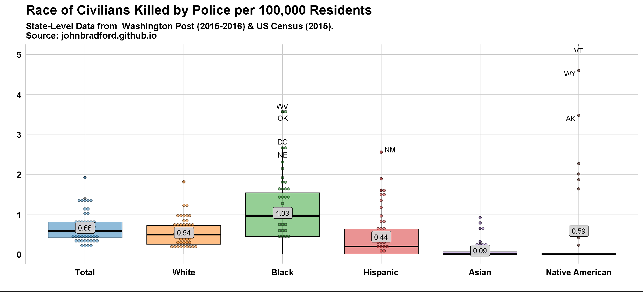
These results contravene those of Shane, Lawton, and Swenson (2017) and are well known. I thought that maybe they had calculated their mean fatality rate using total population rather than race-specific population as the denominator. This seems doubtful. Re-calculating using total population as the denominator, the White rate is higher than the black rate, but the results are still far off. My results are 0.37 white killings per 100,000 people (of all races) and 0.14 killings of blacks per 100,000 people (of all races), rather than 0.74 and 0.63, respectively. Moreover, I could not replicate the ‘mean fatality base rate’ of 0.897 for Hispanics.
Was this a mistake on their part, or did I miss something?
jhbradford